Mathematics, An Introduction

Calculator by Jake and Lindsay Sherbert CC BY

Mathematics is extremely important in all of our daily lives whether we know it or not. However a lot of students have trouble with mathematics, and this can happen for a variety of reasons. It may be boring, listening to new rules and formulas that have no conceivable use in reality, often directly leading to the second problem. If a student-regardless of whether they’re a pre-schooler or working on their PhD-doesn’t have a firm enough grasp on older materials, the new stuff will get increasingly more difficult over time. And this is never more prevalent than in math.

I will now begin to describe the basics of mathematics, from basic counting through to the areas of arithmetic, algebra, geometry, and calculus. This will thus be an extremely quick lesson, but I hope it will nonetheless be of value, if only for you to better understand my method for the more complex information that will come later.

Starting with the very beginning, we have the numbers. There are a variety of different systems of numbers used across space and time, however the most common are the Arabic numerals shown below:

0 1 2 3 4 5 6 7 8 9

Every number, no matter how large or small, is composed of these basic building blocks. When you are counting things individually, “one-by-one” or more precisely unit-by-unit, you are moving incrementally along the above line, using 0 or zero if nothing is there at all. Remembering the above order is crucial, as it is used in building larger numbers:

10 11 12 13 14 15 16 17 18 19 20 21 22 23

As you saw before, the numbers 0-9 are first written individually, but in order to make larger numbers they are required to combine. First the number 1 is placed in front of each of the others, and then 2, 3, and so on, until we reach 99. At this point you repeat the previous process over again but on a higher level, starting with 100, 101, 102…through to 109, 110, 111, 112…all the way to 199, 200, 201…and then 999, 1000, 1001…in a pattern that continues indefinitely.

Numbers are used throughout the world, and not just for simple unit-by-unit counting as seen above. This is where the study of quantity, or arithmetic is used. Arithmetic involves the operations used in combining or separating groups of numbers. The most basic operation is addition, from which all over forms can be derived. Two numbers are added together as follows:

2 + 3 = 5

The + indicates addition between two numbers. Looking at the list of numbers above, you can see the number 2. Move three units away from zero past 2 and you’ll get 5. The = is the equals sign, and it indicates that everything on the right(in this case the addition of 2 and 3) and on the left(in this case the number 5) have the same value. Now let’s look at the other basic operations at work:

7 – 5 = 2

2 × 4 = 8

9 ÷ 3 = 3

The first is subtraction, which is addition in reverse. In the example used, you find 7 on the line and move five units towards zero in order to get 2. The next is multiplication, which is a basically a series of additions. In the example we are looking for the result of adding four 2‘s (or two 4‘s) together, which is 8. And finally, division is the opposite of multiplication, instead asking how many 3‘s added together will result in the number 9(which unlike multiplication cannot be done the other way around). It is best to remember like this rather than to memorize large multiplication tables, because it allows you to better see how the numbers all fit together, in addition to saving time. There are several easily recognizable patterns that can arise through this method(ie. 2 × 10 = 20, 3 × 10 = 30) and it allows you to better understand how zero works(try figuring out why 5 × 0 = 0 or 0 ÷ 6 = 0 using my above explanations).

A further use for division is fractions. The example 9 ÷ 3 = 3 can also be written as 9/3 = 3, with 9/3 being the fraction. Aside from division, fractions can represent the different parts of a larger number, such as one half(1/2) or three-quarters(3/4). Some fractions are illustrated below as segments of circles, each of which represents a whole number, in this case 1.

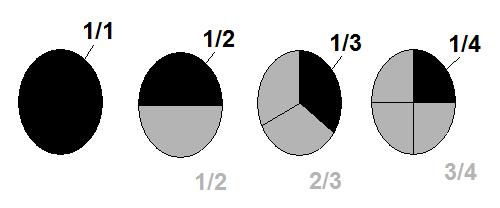
No matter now much we break up the circles, their parts will always add up to one. One half(1/2), or one part of two, added to another half makes two halves(2/2), or two parts of two. But rather than keep it in this form, we would use division again in order to simplify: 2 ÷ 2 = 1. Likewise:

 1/3 + 1/3 + 1/3 = 3/3 = 3 ÷ 3 = 1

1/4 + 1/4 + 1/4 + 1/4 = 4/4 = 4 ÷ 4 = 1

Fractions are proper if the numerator on top is less than the denominator on the bottom, indicating a value between zero and one. They are improper if it is possible to further reduce them, as is the case with 2/4, which can be reduced to 1/2(and from the images above we see that they are indeed of equal size) by dividing both the numerator and denominator by the same number, in this case 2. 9/3 is also improper, being further reduced to 3/1 or simply 3. In the case of 8/3, keep in mind that this is still division as explained earlier, so that within eight units, only two 3‘s can add together, leaving 2 as a remainder. Thus, 8/3 is reduced to 2 & 2/3.

In addition to fractions, numbers can also be written in decimal format, which will include the whole number(even if it is zero), followed by a decimal(.) and the fractional amount. A good way to start seeing how this works is to compare the multiples of 1/10 compared to their decimal(wherein “deci-” means 10) forms, and to deduce the rest from there. In some examples I’ve put fractions into improper forms in order to make 10 the denominator.

1/10 = 0.1, 2/10 = 0.2, 3/10 = 0.3, etc.

1/5 = 2/10 = 0.2,  1/2 = 5/10 = 0.5, 4/5 = 8/10 = 0.8

7/5 = 1 & 2/5 = 1 & 4/10 = 1.4

All the equations used up until now contain numbers that were already known to us, but as we go further we have to explore algebra, which introduces letters as placeholders for unknown numbers, commonly referred to as variables. For instance, to use the earlier adding example, 2 + x = 5 has now been turned into an algebraic equation. We of course know that x = 3, but let’s stay with the problem to see how we can better isolate x.

To do this, you have to do the same operation on both sides of the ‘equals’ sign, because in order to remain equal, anything done to one must be done to the other(as seen before with altering fractions). So, what series of operations can you perform to make 2 + x into x? Let’s try subtracting 2:

2 + x – 2 = 5 – 2

x = 3

But we already knew that, right? The same thing can be done using any of the other operations, so try it out! These types of equations are quite easy to perform if there is only one unknown number, but things start to get trickier once more variables are introduced:

a + b + c, 2 × (a + b)

(b × h) ÷ 2, a × b 

The above expressions each have more than one variable, making them impossible to solve on their own. Thankfully these are equations that are related to shapes in space, meaning that we will be able to obtain some or all of the variables by measurement. This is the next subdivision of mathematics, known as geometry. The top two expressions can be used to determine the perimeter, or complete path around, of a triangle or rectangle respectively. The bottom two are used to calculate the area within each of these shapes. a, b, and c are the sides of the shapes, while h  refers to the height of a triangle from b to the opposite corner while forming a right angle(which will be explained soon).

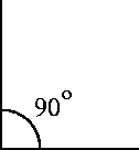These each have a constant number of sides, which define the name of the shape. A triangle has three and a quadrilateral four, a pentagon five and so on. They can be defined even further by their angles. An angle is the corner between two lines, in this case the sides of the given shape. A quadrilateral for instance has four angles, the sizes of which determine the type. The 90° angle is called a right angle, and a quadrilateral possessing four of these is called a rectangle(furthermore, if it has four right angles in addition to four equal sides(ie. a = b = c = d), then it is called a square). Other types of angles include acute(less than 90°), obtuse(between 90° and 180°), straight(180°), and reflex(greater than 180°).

The shapes shown so far are two-dimensional, but there also exist three-dimensional objects, along with a new method of measuring them known as volume. Here are a few examples:

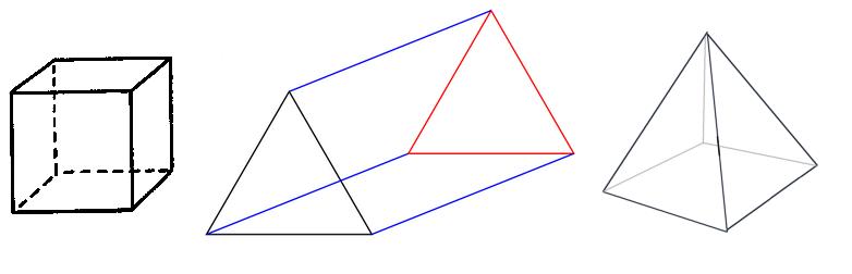The two on the left are both prisms, one rectangular and the other triangular. Their volumes can be calculated simply enough, by taking the area of one of the two equal faces and multiplying by the distance between them. The third object is a pyramid, whose volume is equal to the area of the base multiplied by height, and then divided by 3. For example:

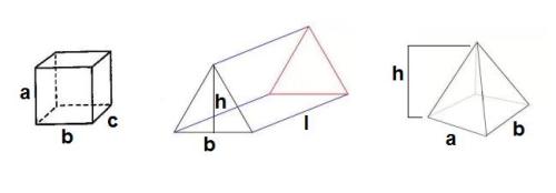
Using the variables given, the volume of each object can be shown by the equations a × b × c, (b × h × l) ÷ 2, and (a × b × h) ÷ 3, respectively. Notice that for the prisms we’re just using the equations for area from earlier while including an extra dimension, such as l in the triangular prism’s case. For the pyramid we start to calculate the volume just like we would the prisms, but we then have to then divide by 3. This is because a pyramid has exactly 1/3 the volume of a rectangular prism with the same base and height.

But let’s go back to the rectangular prism for a moment. Unlike the triangular variant, it is less obvious which two faces were the bases for the equation, right? This is because you could take any two opposite faces and consider them the bases. In the equation a × b × c, any of the three variables could be the length, with the other two representing the area of the base.

Going one step further, if a = b = c, then we have a cube, a special case where all six sides of the object are equal(or in other words, squares). Thus the area of each side could be written as a × a while the volume of the cube could be a × a × a. However in practice we instead take the number of equal variables and place them in a superscript known as an exponent. To illustrate:

a × a = a²
a × a × a = a³

Now let’s try to replace these variables with numbers again for a moment. If a = 3, then a² = 3² = 3 × 3 = 9. This means that a square with 3 units on each side will have 9 units overall. Furthermore, a cube where a = 3 will consist of 3³ = 3 × 3 × 3 = 27 units. But aside from squares and cubes, you can also have a⁴, a⁵, etc., and even a^1/2, which is more commonly seen as √a and known as a square root. Just like division is the reverse of multiplication, the square root is the reverse of the square. For example, if 3² = 9 then √9 = 3. Similarly, you can also have a cube root and even a quarter root, but we’ll stick with the square ones for now.

These new methods of counting start to get very convenient as we expand our scope one step further, and include another dimension, time, as we explore the last main division of mathematics: calculus, the study of change.

To understand calculus you must first understand functions. Consider a variable x which, for any possible value it could have, there exists a unique variable y to correspond to it. That is, y is a function of x, or y = f(x). For example, if x was velocity and y was distance traveled, there would be an obvious connection between the two, and no two velocities would yield the same distance traveled. These results could then be plotted onto a graph, complete with two number lines called the x-axis and y-axis, both representing every possible value these variables can have. The spot where the two axes meet is known as the origin, which is where both x and y are equal to zero. Here are some examples:

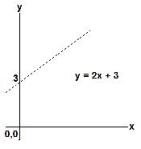
These three graphs represent linear functions, which are aptly named because they are all straight lines. The first graph is pretty straightforward, no pun intended; for every value of x, y = 7. Thus, it is a line that makes a right angle with the y-axis. The others however have y increasing in value the greater that x becomes. All three lines can be written in the form y = mx +b, where b is the y-intercept(ie. the point where x = 0) and m is the slope, or rate of change of the line. When the slope is not so obvious, it can be calculated by taking the change in value of y(written as Δy) divided by the change in value of x(written as Δx) between two points along the line. For example, in the y = 2x + 3 graph between the origin and x = 1, y would have changed from 3 to 5, while x would change from 0 to 1. Thus:

m = Δy ÷ Δx

m = (5 – 3) ÷ (1 – 0) = 2 ÷ 1 = 2

The next logical step forward would be to move on to nonlinear functions, but that will first require going back through the variety of mathematical topics touched upon here and further expanding on them. And that is the goal for next time, when I hope to see you return.

The Enemy From Within, 2500-2000 BCE

Figure 1: The world’s oldest dock in Lothal, one of the Indus Valley Civilization.’s largest cities.

Several great civilizations had already become established around the world, including the originals found in Mesopotamia, the Indus Valley, China, Egypt, and Norte Chico. From these birth grounds, the ingredients of civilization began spreading further across the globe: across the Mediterranean from Egypt through Canaan and Turkey into Greece, home of the Minoan civilization, the oldest in Europe; from China into Southeast Asia where the Hồng Bàng Dynasty was founded in modern Vietnam; and into the Iranian plateau where the Elam civilization developed from Mesopotamian influence. The influence of these already great cultures would slowly creep through the rest of the world, much of which was still the home of hunter-gatherer populations. This would happen through the creation of trade networks across the land, but also as a result of the growing ambitions of those who sought to spread their influence by force. This allowed for greater security across growing empires, while at the same time making them more susceptible to the enemy from within.

Figure 1: The Great Sphinx

There remained a large degree of peace in Egypt during the Old Kingdom, due in large part to the stable government that was in place, in addition to the absence of any serious threats coming from outside its borders. The Egyptians were at the time much more advanced than their nearest neighbours, and they carried out a number of military expeditions into Libya, Nubia, and Canaan. With this prevailing peace came an excellence in art and architecture, as already seen from of the pyramids. But by 2500 BCE there was even more to admire with the construction of what remains the largest monolith statue in the world, the Great Sphinx. The project was orchestrated by Khafra, the son of the now late Khufu, it what would become the oldest known monument in the world.

Figure 2: Ship from Egypt

The Egyptians held trading expeditions to foreign lands, building massive ships in order to sail through the sea. Their ships were built with Byblos cedar and held together with rope and plant matter, and were most likely used on their journeys to the land of Punt. The location of Punt has never been confirmed to this day, though it is expected to be somewhere near the southern boundary of the Red Sea, with possible candidates being modern Somalia, Djibouti, and/or Yemen. It was here where they traded for many valuable commodities, such as gold, ivory, and wild animals.

Figure 4: Collection of seals with Indus script

It is possible that the Egyptians traded as far afield as the Indus Valley, where an extensive trading network was being put together. The Harappans had their own boats for transport, with canals and docks being found along the coastline. The oldest dock found in the world in fact comes from Lothal, a seaside community in modern Gujarat. It was originally a small village before being destroyed by floods, at which point the Harappans expanded it during reconstruction, while also constructing a dockyard for the purpose of trading. It was also by this time that the Indus script was first used, the earliest writing in the region that consists of over four hundred characters and that is still undecipherable by today’s scholars. Among their writing include images, mainly of local wildlife in addition to what may be the earliest known depiction of the Hindu god Shiva.

Meanwhile in Mesopotamia, two distinct cultures were becoming evident: the Sumerian city-states to the south, each competing with each other over power and influence, and the Akkadians, a Semitic people from the north. Taking advantage of their disarray, Sargon the Great commenced his conquest of Sumer in 2271 BCE with the Battle of Uruk. His attack on the city was successful, leading him to tear the city to the ground. This turn of events finally caused the remaining city-states to unite under the leadership of Lugal Zagesi of Umma, but it was already too late. The Sumerians were completely defeated, and the Akkadian Empire, the first of its kind in the world, was born.

Figure 5: Sargon the Great

The empire was ruled from the capital of Akkad, a city which had yet to be found though it is rumoured to be beneath modern Baghdad. From here, the Akkadian language spread throughout the empire, quickly replacing Sumerian as the lingua franca in the south. To further secure his power, Sargon replaced the leaders of the Sumerian city-states with his own soldiers, who had already proved their loyalty to him. As his sons succeeded him, the empire’s reach spread even further, pushing the Elamites further east while also conquering lands to the north and west all the way to Anatolia. The empire was at its largest under the rule of Naram-Sin, and remained as such for nearly one hundred fifty years.

In the Americas, the Norte Chico remained the only prominent civilization of the time, meaning that they did not have to contest with threats from outside their borders like their Old World counterparts were. They were a seemingly peaceful people with no indications of weapons or war, however they did have religion. The oldest religious icon in the Americas has been dated to 2250 BCE in this region, and consisted of a humanoid figure holding a staff in one hand an a snake in the other. The Norte Chico were the only independently formed civilization in the world that was based around the fishing industry instead of agriculture. Nonetheless people were still growing cotton for use in fishing nets, and it was for this reason that communities started being found further inland. They built irrigation canals to assist in farming the cotton, which in turn was used to make clothing, as well as fishing nets. The farmers and fishers were thus dependent on one another to make a living, farmer providing the means to catch the fish, and the farmer providing a food source for the cotton producers.

By 2200 BCE the world’s civilizations were advancing rapidly, but that all changed just as quickly due to a worldwide aridification event. This led to a massive drought spreading through much of the ancient world and lasting for a century, ultimately leading to the collapse of the Old Kingdom of Egypt, the Akkadian Empire in Mesopotamia, and the Indus Valley Civilization, while large floodwaters were meanwhile sweeping the Chinese countryside.

In Egypt the drought prevented the Nile from providing its seasonal floods, thus resulting in a period of famine and disease. The pharaohs were unaccustomed to such disasters after centuries of prosperity, and wealth was already seriously diminished as a result of all the grandiose pyramid and monument building. The influence of power was also much less centralized in earlier times, with the ever growing following of the Sun God Ra. By the time the drought began, more sun temples than pyramids were being built, leading to a decline in the pharaoh’s divine status. In the end, the kingdom was unable to sustain itself, ultimately collapsing in 2181 BCE as Egypt entered a dark period lasting for over a century. Without a central power base, a number of independent states began rising throughout the region, each vying for control over the whole area. Artwork and statues depicting the rules of the old kingdom were destroyed, as Nubia and Sinai both broke away from the crumbling kingdom. Eventually two power centres came into prominence, one in Hierakonpolis in Lower Egypt, and the other in Thebes in Upper Egypt.

The Akkadian Empire was being bombarded with outside attacks, as its leader Shar-Kali-Sharri was unable to defend his inheritance. After his death in 2198 BCE there was a power struggle over succession, during which time a number of former Sumerian city-states were able to reestablish their independence. However their successes were short lasted, as by 2154 BCE the region was invaded by the Gutians, originating from the Zagros mountains in Iran. The Akkadian Empire was already suffering from a period of decline to the drought and shaky leadership which was unable to defend itself. The Gutians deployed hit-and-run tactics that crippled the Akkadians, eventually shrinking the size of the once great empire all the way to the gates of Akkad. It was essentially reduced to a city-state, with two more leaders of Akkad being recorded before the city was completely destroyed in 2115 BCE, where it remains lost to this day.

Figure 6: Yu the Great

In the Indus Valley, the Harappans began abandoning their cities in drought-ravaged regions in favour of less arid regions of the Indian subcontinent. The third Hồng dynasty was meanwhile ruling in Xích Quỷ, which was now renamed to Văn Lang as the capital was moved to Phong Châu, in modern Vietnam’s Phú Thọ Province. In China, the Yellow river was plaguing the region with floodwaters, leaving Gun, a descendent of the Yellow Emperor, tasked with finding a solution. He dammed up the river, and was successful for a time, but ultimately the waters proved too strong. His son Yu eventually took over the project, examining his father’s failures while coming up with a new solution. He finally drafted a series of irrigation canals meant to bring the water back out to sea, commencing a project that would last thirteen years.

During this time Yu refused to return home, despite his having a wife and newborn child. He put aside his own interests in order to help the entire community, and after thirteen long years he was finally successful. And with the land no longer being destroyed by the excess water, he was able to help his people further by aiding in the development of the land, by planting crops and breeding animals.  This made his tribe grow stronger, as territory and influence expanded into neighbouring regions under his leadership. This life of dedication to his people finally earned him the throne, a position that he initially declined. He later accepted the offer however, making his capital at Anyi in modern Shanxi province. Yu began a trend of royal hereditary, with kings being chosen based on blood rather than capability, and thus the era of Chinese dynasties was born. In 2070 BCE Yu became the founder of the Xia Dynasty, the oldest of its kind in China.

Figure 7: Mentuhotep II

Around the same time in Egypt, the two main rivals were still fighting for overall control, when the ruler of Lower Egypt was killed while attempting to conquer new territory. This was the chance that Upper Egypt needed, as leader Mentuhotep II began his slow annexation of the north.  By 2050 BCE Egypt was finally reunified, giving birth to the Middle Kingdom. Mentuhotep II made Egypt strong again, retaking the Sinai while holding a number of campaigns against Nubia in the south and Canaan to the east.

In Mesopotamia, the new Gutian rulers, nomads by trade, were finding themselves unaccustomed to the Sumerians’ civilization, and incapable of agriculture or irrigation. This resulted in widespread famine, which weakened the region for decades to come. Finally, in 2047 BCE, the Sumerians were at long last able to overthrow their oppressors, with Utu-hengal being the first Sumerian king after over two hundred years of foreign rule. But it was Ur-Nammu who would create the new ruling dynasty, the Neo-Sumerian Empire, with its capital of Ur. It encompassed a much wider area than before Sargon of Akkad ever sets his sights on it, spreading from Semitic Assyria to the north all the way to Elam, a region quickly captured by the Sumerians after its own quick collapse at the hands of the Gutians.

By the end of the millennium in Greece, the Minoan civilization was flourishing, eventually enveloping the nearby Cycladic peoples as a vast Mediterranean trade network. Their architecture was rising in prominence with the construction of palaces across their realm of influence, as the earliest and perhaps most famous stories of Greek mythology were being written. And they weren’t alone in their prosperity, as the new Egyptian Old Kingdom, Neo-Sumerian Empire, and Xia Dynasty began to thrive after finally breaking free from environmental hardship. The future seemed bright, but with the knowledge of how things had been, it could only represent the calm before the storm.

To be continued in Part 6: The Calm Before The Storm

Figure 1: Lothal dock by Rama’s Arrow CC BY-SA

Figure 2: Great Sphinx 2010 3 by Wknight94 CC BY-SA

Figure 3: Gizeh Sonnenbarke BW 2 by Berthold Werner CC BY-SA

Figure 4: IndusValleySeals by World Imaging CC BY-SA

Figure 5: Sargon of Akkad by Iraqi Directorate General of Antiquities CC0

Figure 6: King Yu of Xia by National Palace Museum, Taipei CC0

Figure 7: MentuhotepII by Metropolitan Museum of Art CC0

The Making of Legends, 3000-2500 BCE

Figure 1: Great Pyramid of Giza, built during Ancient Egypt’s Old Kingdom circa 2550 BCE.

In my last entry, I discussed humanity’s quickening acceleration from a society of farmers into some of the first civilizations that the world has ever known. They centred around many of the world’s greatest rivers, including the Nile, where people fled to after the desertification of the Sahara, allowing the Naqada  culture to thrive, eventually encompassing what would become Ancient Egypt; the Tigris and Euphrates, home to Ancient Mesopotamia, and the oldest cities in the world, where people from various walks of life came together to create a thriving community; the Indus, around which many large cities began to form, including Harappa, an advanced community which is home to the earliest known writing in the region; and the Yellow and Yangtze, where Chinese culture developed, bringing with it many traditions and customs that are still very much in practice today.

These civilizations were the first the world had ever seen, and it was still just the beginning. Writing was being developed in each of these societies, allowing more to be unearthed about the individual people, from the merchants involved in trade between communities, to the warriors concerned with protecting their homes and families, and to the leaders of the empires and dynasties themselves. Furthermore, creation theories, religious doctrines, and various other theologies were coming into existence, in what would be a time saturated with the making of legends.

Figure 2: Isis, in bird form, copulating with the resurrected Osiris

In Ancient Egypt, a variety of creation myths existed among the different communities present before unification. They all tend to tell the story of a world covered in water, an eternal sea of chaos. And from the sea, the land of Egypt arose from where before there had been nothing, and out of the land came the sun. The sun, often representative of the god Ra, rises above giving both light and warmth to the land and the people who call it home. Ra also becomes the first king of these people,  bringing stability to the land, flooding the Nile annually to allow the crops to grow, and protecting the people from the chaos represented from the demons of the desert beyond. Another common myth, and perhaps the most famous, is the one of Osiris. Killed by his brother Set in order to take over the throne, Osiris was cut into several pieces and spread across Egypt. At this point Osiris’ sister and consort, Isis, found all but one of these pieces, replacing the missing penis with a golden phallus. She then breathes life back into him for a short time, conceiving a son with him before he is sent to the underworld to become the ruler there. Their son, Horus, eventually comes of age and challenges Set for the throne that is rightfully his.

Figure 3: Mastaba in Saqqara

And after a long battle between them, several accounts conclude that their realm was divided in two, becoming what was known as Upper and Lower Egypt, generations before they were reunited by Narmer. All subsequent pharaohs were said to be descended from the gods, particularly Osiris and Horus, and consequently have the highest authority in the land, as head of the army, the priesthood, and the law. And upon death, they would be honoured with a special tomb to spend the rest of eternity within, known as a mastaba. These were rectangular structures with flattened rooves that were constructed with mud brick.

Figure 4: Cycladic female figurine

Across the sea from Egypt, civilization began to arise in the Cyclades Islands within the Aegean Sea separating the modern nations of Greece and Turkey. By 3000 BCE, people were using tin and copper to make bronze, and were also becoming experts at carving stone.  On the islands of Paros and Naxos, figures of women, some of which were life-sized, were constructed from stone and ruled smooth with emery native to the region. Over fourteen hundred of these figures are known, and it has been suggested that they were meant to represent the many goddesses that were believed to look over and protect the deceased. Mainly a seafaring people, the Cycladic culture involved a network centred around the island of Delos, connecting the various islands, each adding their own local commodities to the civilization. Naxos as previously mentioned had a good supply of emery which was used for smoothing stone, while Milos was in possession of the obsidian rock that was used in making knives and scraping tools.

The first literate civilization in Europe were the Minoans of the Greek island of Crete, who were in possession of clay tablets with writings that can be dated to at least 3000 BCE. They were also crafting tools and weapons made from bronze by this time, in addition to houses and royal palaces built from mud bricks. Their religion was important to them, with the most prominent figure being the mother goddess, who was seen as a symbol of fertility. However the Minoans had no great temples to honour her, instead leaving special rooms in their palaces and homes. They also did some extensive trading, with evidence of their pottery being found among the Cyclades all the way to Egypt and Phoenicia.

Figure 5: Remains of Troy

On the mainland of Anatolia in modern Turkey, the city of Troy was founded by 3000 BCE. Originally starting out as a small fortified citadel, only used by local farmers when facing danger, it eventually grew considerably larger and wealthier as time progressed. As a crossroads between Asia and Europe, in addition to its vicinity to both the Black and Aegean Seas, it became an important hub for trade. Over time the community grew in size and wealth, thanks to the extensive trading that was taking place. Furthermore, with its positioning at the entrance to the Hellespont Strait, Troy was able to control marine traffic in the area, making it a key strategic location to surrounding civilizations.

The Phoenicians’ homeland was the coast of today’s Syria, Lebanon, and Israel, and they consisted of merchants, navigators, and skilled boat builders. They were building many great cities at this time, including Ugarit and Byblos, the latter of which became a very important trading port in the region where they would sell their cedar trees and other commodities in exchange for Egyptian gold and Minoan pottery. Calling themselves Canaanites, they became known by their more popular name as a result of their trade of a reddish purple(or “phoinix”) dye used in making clothing.  In addition to this they also loved learning, and are responsible for inventing the alphabet that was soon adopted by the Greeks and became the basis for many other European languages in following centuries.

A little further east in Sumer, rather than being a unified civilization the land was dotted with a variety of city states. Each of these cities had their own patron deities, gods and goddesses which numbered in the hundreds. Of these Nammu is said to be the creator goddess, who made both the earth and the sky, subsequently giving them to the god An and the goddess Ki. Then when these two had a son named Enlil, he was made the god of wind, and thus the messenger between the realms of his parents. More gods would appear over time, bringing life to the world and the people who called it home. Most of these people would lead lives dedicated to the gods, with some exceptional humans becoming lugals, or great men.  Each of the city states in Mesopotamia were run by these lugals, the heads of the warrior class who eventually became the first Sumerian kings. The most famous of these kings was Gilgamesh, who was made into a legendary figure by people of later times. Gilgamesh is credited with building a giant, six mile long wall around the city of Uruk. He was the fifth king to have ruled this city, during a period when the various city states were fighting for more power over one another.

Their influence spread as far as modern Iran, where the Elam civilization was born. Centralized around it’s capital at Susa, it was similar to neighbouring Sumer in a number of ways, including agriculture and the construction of their own massive ziggurats. They were still rivals to the Sumerians however, and there were several conflicts between the two neighbours. This escalated until 2700 BCE when Elam was conquered by Enmebatagesi of Kish, one of the Sumerian city states. This was the beginning of greater Sumerian control in the region, as the Awan Dynasty began to rule over the Elamite people.

Figure 6: Longshan eggshell pottery

Along China’s Yellow River in modern Shandong province, the Longshan culture rose to prominence by approximately 3000 BCE. They were highly skilled in pottery, and utilized potters’ wheels in their design. Their black eggshell pottery was most stunning, being as thin of the shell of an egg while maintaining a bright and beautiful appearance. The Longshan proved better at agriculture than the Yangshao before them as they domesticated more animals, while they had both rice and millet cultivation clearly established. And further south along the Yangtze River the Liangzhu culture was also thriving, adding their jade and ivory creations to the relics of the area. They likewise possessed advanced agriculture, and also aquaculture of the nearby waterways.

Figure 7: Nüwa and Fu Xi

It is at this time in Chinese history that the first known of the great rulers come into power. Over time their stories have been made the work of legends, to the point where their existence in actuality has come into question. For instance, much like the Egyptians, the Chinese speak of a world once engulfed in flood water, with the only survivors being the godlike Fu Xi and Nüwa. They were said by some sources to have been the ancestors of the Chinese people, and the first of the Three Sovereigns and Five Emperors of Ancient China, with Fu Xi beginning his reign circa 2800 BCE.

Figure 8: Huangdi

However Fu Xi has become more of a legend than a historical ruler, leaving Huangdi, or the Yellow Emperor of the subsequent century to have more basis in reality. Huangdi is said to be the founder of Chinese civilization, with credit often going to him for instigating writing, in addition to farming, during which he tamed several wild beasts to assist the people. He is also credited with clothing the people and introducing the Chinese calendar. By 2500 BCE Huangdi fought during the Battle of Banquan in modern Shanxi province, which is thought to be the earliest known large scale battle in Chinese history. It is said that he fought the forces of Yandi, or the Flame Emperor, coming out victorious. The two sides thus made an alliance, and their descendents became the Han people, the biggest ethnic group in China today.

Further south in Vietnam, after over a millennium of rice cultivation, a civilization based around it began forming along the bank of the Hồng, or Red River. There were several smaller territories in the region, but that all changed in 2879 BCE when Lộc Tục began uniting the various nations. This was in order to bring more people together to extract more labour and ability in getting water to the many rice fields, and also to better defend the now unified territory. This was birth of the Hồng Bàng Dynasty, in what would be the start of a new nation known as Xích Quỷ, consisting of much of modern Vietnam in addition to regions of several modern Chinese provinces. Lộc Tục, or Kinh Dương Vương as he was now called, was the first king of the dynasty, and is today considered the founding father of Vietnam.

By about 2793 his son Lạc Long Quân took over the rule of Xích Quỷ, leaving behind a reign which can only be described as legendary. There exist stories from this time of him slaying massive beasts that threatened the livelihoods of his people, including the mythical nine-tailed fox. He was said to be descended from dragons, while his wife descended from fairies, and together they would become the parents of one hundred sons. However, due to the inner conflicts between the two ancestries, it was agreed that husband and wife would separate into opposite parts of the land, each bringing along fifty sons. He went into the rivers of the lowlands while she headed to the mountains of the highlands, expanding their kingdom while the eldest son Hung Lang would rule from the capital.

Figure 9: Stonehenge in England

To the other side of the world in Britain, construction of Stonehenge, the best known example of a megalith structure, began in England circa 2950 BCE. It consists of a centre altar stone, surrounded by two horseshoe arrangements of stone, which itself is surrounded by an outer ring of stones. Bluestone and sarsen were both used in this construction, though the fact that neither is found locally meant that they were transported there in a time before the wheel. There is evidence to suggest that the stones were taken from the Preseli Hills in modern Wales, over thirty kilometres from the Stonehenge site. Part of the journey may have been taken by sea, but nonetheless the Ancient Britons had to transport approximately one hundred fifty stones across such an expanse. Besides Stonehenge, another famous megalith in the area is Avebury, containing three large stone circles that were constructed circa 2600 BCE.

Figure 10: Pyramid of Djoser in Saqqara

In Egypt, the mastabas built to give their pharaohs a safe passage into the afterlife would become the precursors to the first pyramids, which began to arise during Egypt’s Third Dynasty. Built by about 2700 BCE, the Pyramid of Djoser was designed as a final resting place for the pharaoh of the same name, and it consisted of a series of incrementally smaller mastabas built atop one another. Found in the ancient burial site of Saqqara, it is the oldest known structure in history to have been constructed with worked stone, and its design would inspire the creations of the subsequent dynasty.

Figure 11: Snefru’s Red Pyramid

The first true pyramids, those with flattened sides all around, arose in the Old Kingdom, which began in about 2650 BCE. The pharaoh Snefru built the first three of these, the Bent, Red, and Meidum Pyramids. The labour required for these structures must have been immense, alluding to the pharaoh’s pushing into foreign lands to get both workers and building materials. Modeling his pyramids off the earlier Djoser Pyramid, Snefru’s own designs would become the new standard for pyramid construction. However he was only outdone by one pharaoh, his son and successor Khufu, who oversaw the construction of the largest, in addition to the most well known, pyramid ever made, by about 2550 BCE. This was the Great Pyramid of Giza, one hundred forty-six metres tall, and built using roughly two million large limestone blocks. And surrounding the pyramid were several mastabas, intended for high ranking members of the royal court. The entire project must have required massive organization and effort from all over the kingdom and perhaps even beyond, possibly during the flood season when people could not work at home. Roughly eighty-four thousand of these workers constructed this pyramid in a span of twenty years, to create the last remaining wonder of the ancient world.

Figure 12: Harappan pot fragment

The Indus Valley Civilization was spreading from its roots in the modern Punjab region along the Indus River-in addition to a second that is today dried up-and into southern Pakistan and India. Initially they were only a group of farming villages founded by the people who had already been living there for millenia,  but over time agriculture had allowed people to spend more time on less essential activities, and thus different trades began to emerge. Ceramic pots and tools crafted from copper have been found in the area, in addition to faience crafted from partially melted sand. Jewelry consisting of lapis lazuli and turquoise stones was being produced, and this was often buried with the dead.

Figure 13: Remains of Mohenjo-daro

By 2600 BCE the first large cities arose in the region, with populations of up to fifty thousand people in the largest of these, Mohenjo-daro and Harappa. These communities needed to be protected from the floodwaters of the nearby rivers, and were thus either surrounded by large walls or built upon platforms. The plentiful supply of water was used for irrigation, and ports were built along the sea allowing for trade with further regions. There was an elaborate drainage system for sewage material, with a public well present on each city block, illustrating a feat of engineering that has not been matched until modern times. These new advancements in the local societies allowed for people to begin accumulating wealth, and people began to become separated in terms of class with the appearance of new, richer neighbourhoods. The cities became the home of craftspeople who did not participate in agriculture directly, instead making a living off of their art. Necklaces made of long carnelian beads took about a year to make, and were thus extremely valuable, being traded as far astray as ancient Sumer. For those who did practise agriculture, wheat and barley were the main crops, with sesame, rice, cotton, and legumes also being common, and the sheep, zebu, and water buffalo being used for both their meat and milk.

Figure 14: Norte Chico Caral Pyramids

In North America, most people remained nomadic hunter gatherers, migrating across the land on a seasonal basis. The megafauna were now long extinct, and people from one end of the continent to the other were developing different lifestyles in order to adapt to their surroundings. New tools were created, including baskets and nets, and thanks to far-reaching trade networks they were able to spread just as far as the people. Further south in the Caribbean, the Ortoiroid people were continuing to colonize the Lesser Antilles, soon reaching the island of Puerto Rico. And in South America, the Norte Chico of modern Peru, a seemingly peaceful people who had no weapons and thus no need for violence, developed the first civilization to be found in the western hemisphere. They were unique among their contemporary civilizations in their non-violent ways, but also in that they had yet to create any form of pottery, instead using locally grown gourds. Nonetheless they possessed great building prowess, such as in the ruins of Caral, where several buildings, including six pyramids built in roughly the same manner of the mounds found in North America. These pyramids, dated to roughly 2600 BCE, were built by filling bags with rocks and assembling them into the structures that still remain standing to this day.

Civilizations were now appearing across the world, with each of them developing their own unique culture. And with the possible exception of the Norte Chico, they each became forced to look beyond their borders to their friends, or potential enemies, in other lands. This had already become prevalent in Mesopotamia with the various city states building up their borders as the less protected communities simply ceased to exist. And the nomadic peoples of central Asia were becoming a threat to several regions, especially those in the drying up Indus River Valley. In Greece and Egypt as well, defences had to be built up to protect the regions from enemies abroad. Though as some found out, the enemy from within can be just as deadly.

To be continued in Part 5: The Enemy From Within

Figure 1: Kheops-Pyramid by Nina-no CC BY-SA

Figure 2: Abydos Tempelrelief Sethos I. 36 by Olaf Tausch CC BY

Figure 3: Mastaba-faraoun 3 by Jon Bodsworth CC0

Figure 4: Cycladic female figurine 2 by Mountain CC0

Figure 5: Ruins of Troy by David Spender CC BY

Figure 6: CMOC Treasures of Ancient China exhibit – black pottery goblet by Editor at Large CC BY-SA

Figure 7: NuwaFuxi1 by Miuki CC0

Figure 8: Yellow Emperor by 社会历史博物馆 CC0

Figure 9: Stonehenge by thegarethwiscombe CC BY

Figure 10: Pyramid of Djoser by Gary Ku CC BY-SA

Figure 11: Egypt.Dashur.RedPyramid.01 by Hajor CC BY-SA

Figure 12: WLA brooklynmuseum Harappa Fragment of Large Deep Vessel by luluinnyc CC BY

Figure 13: Mohenjodaro Sindh by M.Imran CC SA

Figure 14: PeruCaral01 by Håkan Svensson Xauxa CC BY-SA

The Dawn of Civilization, 4000-3000 BCE

Figure 1: Remains of Eridu in Mesopotamia, argued to be the oldest city in the world.

Once a group of nomadic hunter-gatherers, humans around the world began coming together to grow their own food, in what has become known as the agricultural revolution. Wheat and barley in the Middle East, rice and millet in the Far East, and maize in Mesoamerica were becoming staple crops that soon spread across the countryside, as people were able to worry less about finding food. As farmers could produce more than they could personally consume, communities began coming together to form the first villages, where inhabitants were able to develop sedentary lifestyles. And with this, people around the world were able to leave the task of farming to others as they turned to the task of city building. And soon enough, of civilization building.

In Egypt by around 4000 BCE, several small villages had sprouted up along the shores of the Nile in the wake of the desertification of the surrounding area. One of these small villages was home to the Naqada culture, a small fishing community that, over time, expanded north along the Nile, developing into a vastly powerful civilization in control over the entire region. Nekhen was their power centre, and was at the time one of the largest cities along the Nile. From here they traded their many material goods, including jewelry and faience, with people in the surrounding area. They began using a writing system, which included symbols which would eventually be the precursors to Egyptian hieroglyphics. Their location along the river was ideal, as the annual flooding put water and silt onto the fields, allowing for an abundant harvest every year. This lead to a healthy population, leading to a growth in numbers and thus labour force.

Figure 2: Remains of Ur

By 3800 BCE in Mesopotamia, urban life was becoming more common, as strong signs of political organization were coming into being. Thanks to their long tradition of agriculture, they had the first permanent settlements where people lived throughout the year, and hence the first city states. The communities of Eridu and Uruk each had large temple complexes constructed with mudbrick, and by the end of the millenium there were several of these, each with a different god to serve. These grew increasingly massive over time, with Uruk’s in particular eventually encompasing one third of the city’s total area. Farmers from the surrounding area were devout followers of the gods represented by these temples, and would always bring a portion of their crops produced to their priest. The priest in turn acted as a leader in control of the trade between communities.

Figure 3: Great Ziggurat of Ur

As trading continued and grew in Mesopotamia, new methods for tallying items began to arise. This began with simple pictographs of various items, which eventually evolved into the first phonetic script, or cunieform, by 3400 BCE. The region was soon becoming dominated by Sumer in the south, as Sumerian civilization was thriving and becoming far more complex than the agricultural communities of centuries past. This was in large part thanks to its pioneers in the feats of irrigation, writing, and math, causing them alone to push the civilization into the future. Oxen began replacing humans in pulling ploughs, greatly increasing yields, while bronze was starting to be molded in the region as well. Good organization and exceptional leadership were required to get all of the differing factions of society to work together, and that seems to be exactly what the people had. Massive ziggurats, pyramidal structures with flattened peaks, were constructed for religious purposes in various cities across the region. It is assumed shrines were present at these peaks, wherein rites and rituals could be performed in honour of the local god. There was no central government in place in Sumer, merely small city states each with their own leaders, causing power to often get moved from one community to another over the passage of time. Soon war began to be initiated between settlements competing for power and resources, eventually leading to the rise of the warrior class, intent on protecting their homes. The head of these warriors was known as a lugal, a role which ultimately evolved into the first Sumerian kings. Over time each city in the region was transformed into a miniature kingdom.

Further north in the Eurasian Steppe, stretching from Ukraine in the west all the way to Manchuria in the east, several nomadic cultures were coming into prominence. It was somewhere in this vast grassland where the first horses were domesticated by around 3500 BCE. The Sredny Stog culture based in modern Ukraine is a contender for this title, though their horses were used primarily as a source of meat. The Botai in Kazakhstan are another possibility, who may have originally bred horses for both their meat and milk. The various steppe nomads lived in an area with a rather inhospitable climate, and remained without agriculture until fairly late in their history. The people relied more heavily on animals, especially horses, which, when fully integrated into their lives, made way for a dramatic transition. Once they were used as working animals, horses began to be used for transporting individual people, thus making their masters truly nomadic. Soon villages from one end of the Steppes to the other were being attacked by armed men on horseback, who could easily raid entire communities and escape before anything could be done. Their reputation soon spread across the continent, as they were feared throughout India, China, and Europe.

The first known use of the wheel also comes from this time, with proof of its use being found in Mesopotamia, Russia, and central Europe. Unfortunately it is not known which of these areas, if any, were the birthplace of the invention, but nonetheless each of their capabilities were greatly expanded. In Mesopotamia for instance, the potter’s wheel was being utilized in the creation of pottery, thus making the whole process much more efficient. The first wheeled carts were being used by 3200 BCE, as both they and ploughs were now being built to be carried by oxen possessing more pulling strength than humans. This allowed goods to be produced and transported much more quickly than was previously possible.

In China, the Yangshao culture was continuing to flourish, having several animals and crops domesticated in addition to being one of the first producers of silk. They also had some fine pottery, complete with paintings of various people and creatures, and the earliest copper and bronze objects found in China. Their agriculture and way of life began to quickly spread into other regions, influencing Vietnam’s Phùng Nguyên and later Đồng Đậu cultures. Circa 4000 BCE, rice cultivation began being practiced in Vietnam, as pottery and jade jewelry began to be produced. Trade with the peoples of Oceania was also prevalent, as proven by the introduction of the dingo, native to Southeast Asia, into Australia by 3500 BCE.

Figure 4: Jeulmun pottery

Further north in Korea and Japan, the people of the Jeulmun and Jōmon respectively were living in semi-permanent settlements,  and practicing deep-sea fishing in the surrounding waters. Furthermore the first evidence of agriculture on the Korean peninsula comes from this time, with remains of millet in addition to cultivating stone tools being found in modern North Korea. The pottery in both regions was also becoming more complex in design, with cord- and comb-patterns becoming more prevalent.

On the other side of the Pacific in modern Ecuador, the first known pottery in the Americas was created by the local Valdivia culture by approximately 3500 BCE.  They were perhaps most famous for their Venus figures, various clay-molded representations of what were likely real people of the time. The Valdivia lived in a permanent settlement of houses surrounding a large central plaza, and lived mainly off of agriculture and fishing. And slightly further south along the Peruvian coast, the Norte Chico civilization, the oldest of its kind in the Americas, began its rise by 3200 BCE. The area consisted of four coastal valleys, where over fifty rivers existed, pushing water from the Andes down to the Pacific Ocean. This allowed the Norte Chico to practice widespread irrigation which ultimately led to the rise of their civilization. They however were without pottery unlike their peers of the Old World, and of the Valdivia to the north, and they remained a society primarily reliant on fishing.

Figure 5: Watson Brake mound

In North America, the people remained part of a hunter gatherer society, though even without forming a civilization like what was present in other corners of the planet, they were nonetheless capable of well-organized contruction. This was made evident by the presence of several large mound complexes created across the continent, with the oldest known being Watson Brake. Located in today’s southwestern United States in the state of Louisiana, Watson Brake is an arrangement of eleven mounds, ranging from one to nearly eight metres tall, and having been dated to about 3500 BCE.  This complex was likely used as a base for nomadic hunter gatherers during the warmer months of the year, who enjoyed a plentiful source of food from the local floodplain of the Ouachita River.

Figure 6: Harappa

Back to the Old World in modern Pakistan, the Indus Valley Civilization began to rise to prominence by about 3300 BCE. The local residents had domesticated the water buffalo, in addition to a number of crops including peas, sesame seeds, and dates. Several of their communities have been unearthed along the shores of the now dried up rivers, with one of the most prominent being Harappa, found in Pakistan’s Punjab province. The civilization appears to have its roots in this region, which also saw the earliest known Indus script, having been dated to 3000 BCE. However, to this day their words remain undecipherable, leaving their historical records lost to the ages.

Figure 7: dwelling of Skara Brae

Europeans were yet to create a great civilization like their counterparts in Africa and Asia, but their trading circles were growing along the coast of the Mediterranean, leading to vast networks that were key in the spread of agriculture. The Linear Pottery culture of the region bred cattle more than any other animal, and were among the first people to also use the animal’s milk. They and others in the network initially grew and harvested their crops of wheat and barley as a part-time process, but as it became more prevalent in their way of life did it become a primary part of their network. A good flint trade had also developed, allowing for better tools, and animals were beginning to be harnessed for pulling ploughs and wagons. Agriculture was now well established across Europe, with the final regions to make the change being Normandy and the British Isles near the start of the millenium. And by 3100 BCE it was definitely present in Scotland’s Orkney Islands, proven by the remains of a herding society at the Skara Brae site unearthed there. The community was a small one with only ten houses, wherein pottery and stone-crafted furniture has been discovered.

Figure 8: Newgrange monument

In addition to the Carnac Stones in France, other large megalithic sites began to both appear and grow across Europe at this time. This included large tombs, created by rolling large boulders together to form walls which were then mounded over with flat stones and finally earth. These constructions were meant to be burial tombs, with some found containing hundreds of people. In addition to these several monuments were found across the British Isles, with Newgrange in Ireland being one of the most well-known. Covering forty-five hundred square metres of land, it houses a chamber where the light of the sun rushes in annually on the winter solstice, the shortest day of the year. Assumed to have religious significance, it may have alerted people to the commencement of longer days. Similar, albeit smaller sites exist around the Isles, such as Bryn Celli Ddu in Wales, which marked the summer solstice.

Figure 9: replica of the Sweet Track

In modern England, what are expected to be the oldest roads in the world, the Post Track and the later Sweet Track were constructed in circa 3900 BCE, consisting of crossed wooden poles used to support a flattened wooden surface for walking. Furthermore in the region, the initial construction of perhaps the most famous of the megalithic sites, Stonehenge, was getting ready to begin.

Figure 10: Ġgantija temple in Malta

To the Mediterranean, on the island of Gozo in modern Malta, the megalithic temple of Ġgantija was initially constructed by around 3600 BCE. It was built with large limestone blocks in a time before the wheel was utilized, leaving local folklore to suggest that it was the work of giants. As one of the oldest religious structures on the planet, and the oldest free-standing structure still in existence, Ġgantija was presumably built by members of a fertility cult wishing to worship their now unknown gods.

Figure 11: Narmer, the first pharoah

And to the other side of the sea, Ancient Egypt was home to several small kingdoms, gradually becoming divided between two cultural regions, Lower Egypt and Upper Egypt. Lower Egypt encompassed the Nile Delta and surrounding areas, while Upper Egypt was further south and had the city of Nekhen as its capital. However by 3100 BCE, the kingdom of Ta-Seti in Upper Egypt was invaded by Lower Egypt, and was ultimately destroyed. This unified the two Egypts for the first time, in what would become the opening actions of a long lasting dynasty. Narmer, the man responsible for the invasion of the south, became the first pharoah, wearing the crowns of both Upper and Lower Egypt and thus having more power than any person before him. He solidified his control by creating a capital in Memphis, on the opposite side of the river from modern Cairo. It has been recorded that Menes was instead the first pharoah, it should be noted, but there remains uncertainty as to whether he and Narmer are one in the same. Nonetheless, all subsequent pharoahs were said to have been chosen by the gods, and consequently have the highest authority in the land, as head of the army, the priesthood, and the law. And upon death, they would be honoured with a special tomb to spend the rest of eternity within, which began as relatively small mastabas, but soon evolved into the great pyramids that the region is still known for today.

The civilizations of Ancient Egypt, Mesopotamia, and the Indus Valley were all in their initial stages at this time, as cities began to grow, and societies began to flourish with innovations which had never been seen before. And at the same time, even more civilizations were growing from communities elsewhere in the world, from the Norte Chico in South America, to the peoples inhabiting the lands in and around the Aegean Sea surrounding Ancient Greece, and to the Three Sovereigns and Five Emperors of Ancient Chinese civilization. With writing now arising in most of these places, more light can be shone onto their cultures, religions, and in fact people, most notably leaders. And with this ability came the beginnings of many stories, of legends, which would ignite the imaginations of millions.

To be continued in Part 4: The Making of Legends

Figure 1: Эриду by Таис Гило CC0

Figure 2: Ur-Nassiriyah by M.Lubinski CC BY-SA

Figure 3: Ancient ziggurat at Ali Air Base Iraq 2005 by Hardnfast CC BY 3.0

Figure 4: Korea-Neolithic.age-Pot-01 by Good friend100 CC0

Figure 5: Watson Brake Gentry Mound by Thomas Eubanks, courtesy of the Lousiana Division of Archaeology CC0

Figure 6: Ancient Harappa Civilisation by Shefali11011 CC BY-SA

Figure 7: Skara Brae house 1 5 by Wknight94 CC BY-SA

Figure 8: Newgrange by Shira CC BY-SA

Figure 9: Sweet Track replica by Geoff Sheppard CC BY-SA

Figure 10: Ggantija Temples (1) by Norum CC BY-SA

Figure 11:  NarmerPalette-CloseUpOfNarmer-ROM by Keith Schengili-Roberts CC BY-SA

The Agricultural Revolution, 10000-4000 BCE

 

Figure 1: Göbekli Tepe, built by hunter-gatherers near the onset of the agricultural revolution.

 

Last time, I discussed the evolution of the human species over thousands of years. From our humble beginnings in Africa, homo sapiens spread to all the major landmasses on the planet in just a few thousand years. Our closest cousins on the evolutionary line, homo erectus, homo neanderthalensis, and finally homo floresiensis, became extinct one after another, leaving us as the sole remaining member of the genus. Humans around the globe practised a hunter-gather lifestyle for millenia, developing different types of art and tools along the way, from the Gravettian Venus figures that spread across the European continent, to the cord-patterned pottery of the Jōmon people in Japan, and to the spear points of the Clovis culture in North America, so well-designed as to drive the mighty mammoth to extinction.

But the lifestyle that these people had known for thousands of years, if not tens of thousands, was quickly coming to an end. People once accustomed to a nomadic way of life, traveling from one region to another in order to find food, began producing it for themselves. They began growing various crops, and domesticating the local fauna for both food and labour. It was the rise of agriculture in many locales around the world. It was the agricultural revolution.

Figure 2: Ancient Jericho dwellings

The earliest form of agriculture comes from ancient Mesopotamia in modern Iraq and surrounding countries, dating from 10,000 BCE. These Mesopotamians lived in tiny mudbrick houses for most of their lives, and even in death, after which they would be buried beneath the floor. One of the oldest cities in the region, and in fact the world, is Jericho in present-day Palestine, dating back to 9000 BCE. The residents of these communities grew barley and oats, and created the oldest granaries for which to store their products. The earliest domestication of animals also comes from this era, with the goat and the sheep being used for the first time. It is also likely that the first aurochs were tamed in the area, eventually becoming the descendents of all domestic cattle in the world today.

Figure 3: Göbekli pillar

There was still a partial hunter-gatherer lifestyle for many despite the new innovations, as characterized by the Göbekli Tepe sanctuary in Turkey. Dated from 9000 BCE, it is the oldest known religious structure on the planet, which was presumably used by hunter-gatherers still living in the region. It consists of several large circular structures surrounded by massive pillars containing reliefs of various animals.

Figure 4: Bhimbetka cave paintings

Further east, cave paintings have been found in the Bhimbetka rock shelters of central India, being dated to around 10,000 BCE. They denote images of humans as well as local fauna, including tigers and rhinoceroses. Their dating also indicates the oldest permanent settlements known on the subcontinent, which eventually led to the rise of agriculture in that part of the world. Wheat and barley were domesticated by about 9000 BCE, while sheep and goats, in addition to the first elephants, were also domesticated.

Figure 5: Rock art in Libya

Back in northern Africa, the desertification had yet to begin, and a vast savanna covered the region. This savanna was filled with several species of megafauna, as is proven by the many cave paintings found throughout the area depicting the local wildlife. In the modern nations of Algeria and Tunisia, the Capsian culture, possible ancestors of the Berber people, was present, developing the earliest blade industry in the region, in addition to a variety of art, including jewelry and the aforementioned paintings. Their diet consisted mainly of meat, and signs of their domestication of sheep and related animals have been found.

Figure 6: Rock art in Somalia

In Australia, the Aborigines did not have a plentitide of food and thus did not participate in the agricultural revolution, but nonetheless they were able to adapt well enough to the land in order to find a wide variety of things to eat. They developed boomerangs and spears for hunting the local wildlife, which included kangaroos and emus. They utilized mud to both hide their scent and as a form of camouflage, covering their bodies in it so that they could better sneak up on their prey.

In Europe, the Sauveterrian culture was eventually overrun by the Tardenoisian and Maglemosian cultures, with the former mostly inhabiting France and Spain, while the latter was located in Scandinavia and Britain. They lived in the forest and survived mainly with small tools made of wood and bone. Of note is the near absence of figurative art that was a staple of earlier societies in the area. They also did not practice agriculture for a few more millenia, instead continuing to hunt local wildlife such as the reindeer.

The peoples of the Arctic likewise did not delve into agriculture either, instead remaining hunter-gatherer societies. The Diuktai culture of northeast Siberia moved to Alaska, which was still connected to Russia via Beringia, eventually practising both hunting and fishing as the Sumnagin culture. They became mostly known for their stone technology, including microblades and scrapers used in their tradition.

Figure 7: Folsom point

But for the Americans further south, their way of life was soon coming to an end, as the last of the megafauna went extinct by about 8000 BCE, with the entire Clovis culture going not too long afterward. They were eventually replaced with the Folsom culture, whose main prey included bison and deer.

In the Great Plains, the Plano culture also flourished, replacing the Folsom as the dominant force over time. They made use of technologies to force stampeding animals into running off a cliff or else into a corral for containment. The Plano and their predecessors are notable for their lack of any large cities, instead deciding to live off the land completely. Furthermore, they did not have any form of writing whatsoever, nor even architecture of any kind. Nonetheless the Plano people’s reach was far, with signs of their presence from Atlantic Canada all the way to Chile in South America.

Though they by no means covered the entirety of the Americas, with people flourishing further inland. The Pedra Pintada cave paintings found in Brazil are a good example of this,  revealing the remnants of a culture that did not hunt the larger animals that their contemporaries in North America did, instead adapting to the Amazon environment. One consequence of said environment is that most records of the people living there are lost, with the humid climate destroying all of their materials. So the paintings in Pedra Pintada, indeed the oldest of their kind in the Americas, reveal one of the only glimpses of the people that lived in the area at the time.

Figure 8: Jeulmun  pottery

In East Asia, pottery was beginning to spread to areas beyond Jōmon Japan, hinting at the idea that trade was ocurring between the various regions. Yungimun pottery in the Korean Peninsula dates to 8000 BCE, and the later Jeulmun, or cord-patterned pottery dates to 7000 BCE. While the Jeulmun were still a hunter-gatherer society, they were beginning to practice plant cultivation, albeit on a small scale. It also shares striking similarities with pottery across the region, from Mongolia to Siberia, and of course to Jōmon Japan.

Figure 9: Çatalhöyük figure

Pottery also started being found in Mesopotamia by 7000 BCE, in the northern Iraqi site of Jarmo. As the earliest pottery in the region, it is of a simple design, and it has been found along with clay figures depicting pregnant women expected to be the precursors to future mother goddesses. Jarmo is also known as one of the oldest agricultural communities on the planet, with various crops already domesticated, such as peas, pistachios, almonds, wheat, barley, and lentils. Jarmo was a contempory with Jericho, as well as Çatalhöyük in southern Turkey. Çatalhöyük had many wonderful murals and figurines, often depicting the animals of the area, and women similar to those found in Jarmo. The bull appears to be important to the community, as religious shrine rooms have been found housing the heads of such animals molded into plaster. There is evidence of trade between the two communities, as towns became large enough to support a section of the population who were not primarily involved in producing food. Over time this gave rise to new classes, with the rich and poor becoming the basis for the first hierarchies.

In present-day Mali in Africa, the earliest known pottery on the continent has been found, dating to 9500 BCE. The people of the region also practised agriculture, domesticating various plants in similarly various regions of the Sahara and surrounding areas. Wheat and barley, in addition to the sheep and goat, arrived in northern Africa via Asia, while teff and finger millet, in addition to the first donkeys, were domesticated in the Horn of Africa, watermelons and cotton in the then-savanna of the Sahara, and okra, kola nuts, and black-eyed peas in West Africa. In the southern regions of Africa, however, agriculture did not spread as it did in the north, with the Khoisan and pygmy people there maintaining a hunter-gatherer lifestyle for a much longer time.

The earliest evidence of  farming in South Asia has been found at the Mehrgarh site in Pakistan, where inhabitants grew wheat and barley, in addition to keeping sheep, goats, and cattle. The people lived in mud brick houses, and had granaries like their counterparts in Mesopotamia. They also possess the earliest signs of dentistry, with evidence of teeth drilling dating to 7000 BCE at the earliest. They were also performing flint knapping, bead production, and leather making, while pottery appeared by approximately 5500 BCE, and soon feminine figurines were being created as well.

Signs of farming in Papua New Guinea date to 7000 BCE, making it one of the oldest agricultural centres on the planet. The first domestication of taro, sugarcane, and bananas was in this part of the world, and they were cultivated using irrigation of the land via large drainage ditches. Crops from New Guinea began spreading out to neighbouring regions, initially including Indonesia and the Solomon Islands.

Meanwhile in China around 7000 BCE, agriculture was already becoming well established, while the pig and dog were being domesticated for the first time. And perhaps most importantly, in the Damaidi cliffs, found just north of the Yellow River in the Weining mountains, petroglyphs dated to 6600 BCE have been found. These display 8453 different figures, depicting the sun, moon, and stars, in addition to people hunting and herding the local fauna. Over 1500 of these images resemble early hieroglyphs that would later become Chinese characters, indicating that Damaidi may hold the earliest records of writing in the world.

Figure 10: Peiligang pottery

Similar pictoral characters have been found at the Jiahu site in Henan province of central China, dated to about 7000 BCE. The Peiligang culture of the area farmed millet throughout the region, but Jiahu is unique in that it is the only, and also the earliest, site from which rice was cultivated. The Peiligang also had music, with several flutes, the earliest musical instruments in China, being found at Jiahu. They also have some of the oldest Chinese pottery, some of which too had symbols reminiscent of later Chinese characters. The population of the Yellow River Valley was steadily increasing over time, as the first villages in the region began to be established.

The first signs of agriculture in South America rise from the Amazon Basin circa 6500 BCE. At this time, the local people were cultivating potatoes, beans, and chilies at first. In Central America and Mexico, maize was slowly starting to be bred and domesticated. Meanwhile in North America, agriculture had yet to take root, but complex construction was beginning to take form in the southeastern United States. Large earthwork mounds that can still be seen today were erected in the Lower Mississippi Valley at this time. Hunter-gatherer societies remained quite common nonetheless, though evidence of trading between them was becoming more widespread as time progressed. The people in the Americas still consisted of foraging societies, however, but with trade occurring between different groups.

Figure 11: Samarran figurine

The Samarran culture arose in northern Mesopotamia by approximately 6000 BCE, and was known for well stylized pottery with various figures of animals and geometric designs. It later influenced the establishment of the city of Eridu in the south, along the shores of the Persian Gulf near the mouth of the Euphrates River. Eridu appears to be the earliest settlement in the region, and furthermore seems to have been the result of an amalgamation of three different cultures-the Samarran culture of the north, the hunter-gatherers and fishers, and the nomadic sheep herders. Together they formed what was possibly the first permanent settlement on the planet, along with a complex system of irrigation to maintain their agriculture, including canals built to direct water to populated areas. It shows one of the first instances of people working together under organized labour.

Figure 12: Amsa-dong settlement in Korea

There was also trading present in Japan by 6000 BCE, with the coastal fishers trading their catches with the people living further inland. Pottery, now throughout the islands with the introduction to Hokkaido, meant that everyone could cook and boil their food, thus implementing a new diet. The lifestyle quickly led to population increases, particularly in modern Kanto and Chubu, eventually leading some Japanese to move to mainland Asia, and possibly even America. In addition, the number of stone tools was going on the decline, being quickly replaced with small tools and microblades resembling those found on the mainland, also indicating possible trade between the communities. The Jeulmun in Korea were practicing a similar lifestyle, hunting and fishing, while constructing semi-permanent settlements. Back in Japan, the Jōmon had a swidden type of agriculture, where people would move between fields throughout the year, as opposed to moving between different crops. And by 5000 BCE, their already ancient ceramics were beginning to include figurines in addition to pottery.

Figure 13: Yangshao pottery

On mainland Asia, the Yangshao culture arose by around 5000 BCE in China’s Yellow River Valley. They crafted painted pottery with images of people, animals, and geometric designs, and were also an agricultural community, mostly growing millet, while also cultivating wheat and rice.  They kept a wide variety of animals, though most of their meat still came from hunting and fishing. Among the animals domesticated were the first silkworms, producing silken clothing for the wealthy of society.  Other animals include the water buffalo, chicken, and duck, and domesticated plants include peaches, kiwis, turnips, and cabbages.

Figure 14: Lepenski Vir sculpture

In Europe by 7000 BCE, the Lepenski Vir culture was thriving in present-day Serbia. Their community consisted of one large settlement located on the banks of the Danube river, with several smaller satellite villages surrounding it. Their main source of food came from fishing, which wasn’t very unusual, as it was common to cultures along the Danube. What made the Lepenski Vir unique were their pristine sculptures of fish. But even their hunter lifestyle was quickly coming to and end, as the rise of agriculture began sweeping in from the Middle East.

Figure 15: Linear Pottery vessel

The agricultural revolution moved to Europe by about 6000 BCE, starting in the Anatolia region of Turkey and eventually spreading across the continent. In fact, all wheat currently on the planet can be traced back to a small patch in present-day Turkey. The wheel and plough were both around by this time, thus expanding people’s capabilities. What also spread across the continent and beyond were the Indo-European languages, thought to also have originated in Turkey. At around 5000 BCE, the Greek, Armenian, and Balto-Slavic families of languages diverged from one another, as agriculture spread across the land. The Balkans were completely colonized in this time, and a myriad of different cultures began to sprout up across Europe. Most groups of people living on the continent shared several similarities, such as living in small communities, and relying on a combination of domestic plants and animals in addition to hunting. They also produced pottery, though with the notable absence of the potter’s wheel. As agriculture slowly spread across Europe, the Linear Pottery culture arose along the Danube river in Hungary and Austria, eventually stretching outward. They lived at the same time as the Ertebølle culture in Denmark, which like much of Scandinavia and the Baltic region, remained a community of fishers who did not practice agriculture as their southern neighbours did.

Figure 16: Carnac Stones

Dating from 4500 BCE are the Carnac Stones in France, a series of linear standing stones that number more than three thousand.  And in the more northerly regions of Europe, the Funnelbeaker culture arose by approximately 4100 BCE, finally bringing some aspects of agriculture to Scandinavia. The culture, which was also centred in Germany and Poland, crafted containers with funnel-like tops.

Figure 17: Funnelbeaker pottery

In 5000 BCE, the island of Trinidad was still connected to the South American mainland, allowing humans to easily reach the area. The oldest signs of human presence in the Caribbean islands are thus in Trinidad, which was occupied by the Ortoiroid people originally coming from the Orinocco Valley of present-day Venezuela. They first colonized Trinidad and Tobago, before eventually traveling further up the Lesser Antilles. They were hunter-gatherers, using spear points and stone tools to capture the shellfish which were an important part of their diet. The Greater Antilles were first reached by another nomadic culture, the Casirimoid, who established themselves on the islands of Cuba and Hispaniola by roughly 4500 BCE.

Returning to Africa now, the vast grassland that covered what is now the Sahara, the largest desert in the world, began to become considerably warmer and drier starting in 5000 BCE, with the only habitable areas becoming the banks of the Nile and Niger rivers. Thus people began to move towards these river valleys in large numbers. The Nile valley in particular was much less arid at the time, and full of trees, savanna, and wildlife.

Figure 18: Nabta Playa calendar

A little further south, in what is now the Nubian Desert in Sudan, there was a large basin, the Nabta Playa, that likewise attracted a population to grow around it. These people only lived in the area seasonally, when the basin was full, and practiced a way of life that was considerably more organized then those further north along the Nile Valley. Their villages were planned ahead, and included deep wells that could hold water throughout the year. Furthermore, they are responsible for what is perhaps the world’s first archeoastronomical device, in the form of a calendar constructed of rocks presumably marking the summer solstice.

By 4000 BCE, the Naqada culture began to slowly rise, expanding north along the Nile, changing in just a short period of time from a small fishing community to a vastly powerful civilization. They held a power centre in Hierakonpolis, from where they traded with people in all the surrounding regions. They began using written symbols, which would be the precursors to Egyptian hieroglyphics. Meanwhile in Mesopotamia, Eridu’s prominence came to a sudden end, as urban life became more common, and strong signs of political organization came into being. The first city states, along with the first signs of objects being massively produced, come from this time.

Both Egypt and Mesopotamia were rising to levels the world had never seen before, and they were only just starting the trend. Independent from one another, cities began rising around the world, from the Indus Valley, to mainland China, and to the Peruvian coast. Societies began to become hierarchical with the advent of political organization, and urbanized, with people no longer having to focus so much on producing food, as the now ancient tradition of agriculture was so central to many people’s lives. It was a new dawn for everyone-a dawn of civilization.

To be continued in Part 3: The Dawn of Civilization

Figure 1: Göbekli Tepe, Urfa by Teomancimit CC BY-SA

Figure 2: Jerycho8 by Abraham CC0

Figure 3: GobekliTepeHeykel CC0

Figure 4: Bhimbetka Cave Paintings by Raveesh Vyas CC BY-SA

Figure 5: Libya 5041 Petroglyphs Tadrart Acacus Luca Galuzzi 2007 by Luca Galuzzi CC BY-SA

Figure 6: Laas Geel cow and human by najeeb CC BY-SA

Figure 7: Folsom point by U.S. department of the Interior, Bureau of Land Management CC0

Figure 8: Teeth of a comb pattern pottery3 by Kang Byeong Kee CC BY-SA

Figure 9: Ankara Muzeum B19-36 by Roweromaniak CC BY-SA

Figure 10: PeiligangCulture-RedPotWithTwoEars-ShanghaiMuseum-May27-08 by Captmondo CC BY-SA

Figure 11: FemaleStatuetteSamarra6000BCE by PHGCOM CC BY-SA

Figure 12: Korea-Seoul-Amsadong-Neolithic by Jtm71 CC BY-SA

Figure 13: Banpo bowl by Rosemania CC BY

Figure 14: Lepenski Vir Head by Mazbln CC BY-SA

Figure 15: Linear Pottery 001 by Willow CC BY-SA

Figure 16: Alignement Kerlescan Carnac by Myrabella CC BY-SA

Figure 17: Funnelbeaker1 in Nordisk familjebok CC0

Figure 18: Calendar aswan by Raymbetz CC BY-SA

The Peopling of the World, -10000 BCE

Figure 1: Olduvai Gorge, the “Cradle of Mankind”, expected home of the first hominids.

In order to best predict where the world is headed, it is essential to discuss where it has been. Thus, over the next few weeks and months, I will share what I’ve learned about the progressive history of the planet. Humans have had a relatively short time on Earth, but nonetheless there is a plethora of material to discuss. Almost as difficult as determining what to include was determining where to begin. The rise of civilization, the rise of agriculture, or the evolution of the species? I have decided to begin with the last of these, exploring vast spances of time in mere moments while gradually slowing myself down as the years go by.

Planet Earth has billions of years of history, however humans and related species have only been present for merely a couple million years. The earliest of these hominids are expected to have originated around modern day Tanzania, in the vicinity of the Olduvai Gorge approximately four million years ago. These earliest ancestors of humanity lived a relatively simple existence for another million years, when they began using items found in the natural world as tools-used in collecting food, for instance. A couple more hundred thousand years would pass, and hominids were crafting tools of their own.

Figure 2: Skull of Homo erectus

Homo erectus, one of our closest ancestors, arrived on the scene about one and a half million years ago. They quite possibly became the first hunter-gatherer society the world had ever seen. Initially evolving in Africa, Homo erectus expanded its territory greatly, encompassing  its native Africa and the majority of the Asian landmass including modern day India, China, and Indonesia. Somewhere along this generational journey, Homo erectus also achieved another first with the invention of fire, of which evidence is found in China from around 1.27 million years ago. This ultimately foreshadowed a future of these hominids finally being able to conquer the colder environments of the north, far from the territory that they were familiar with due to their African origins.

But it was not Homo erectus who would achieve this, as another, more intelligent species began to rise to prominence on the African continent. Homo sapiens, or the modern human, evolved at some point between 100,000 and 150,000 years ago, presumably around present Ethiopia, where the oldest known human bones have been found. From there, Homo sapiens expanded their territory as well, though to a much greater significance than Homo erectus before it.

Figure 3: Human skull

The exodus from Africa to Eurasia occurred about 125,000 years ago, with people settling along the coasts of the Arabian Peninsula and beyond. The most likely point of entry into Eurasia appears to be the southern shores of the Red Sea, which would have been considerably more shallow in addition to being littered with small islands. Furthermore, the region was much more fertile in these ancient times, with springs expected to be erupting along much of the Arabian coast, providing all the necessities for the further expansion into distant regions.

While some of these groups moved inwards toward Central Asia, more continued along the coastline, reaching Persia and India. The Indian subcontinent was first reached by Homo sapiens approximately 75,000 years ago, whence their trek through Southeast Asia began. On the island of Flores in Indonesia, humans would have first come in contact with Homo floresiensis, a small, dwarfed Homo species which would coexist with humans for some time.

And by 50,000 years ago, Australia, which was not as secluded as it is today, was reached, thus marking the first time Homo sapiens were able to set foot on a landmass previously unreached by Homo erectus. This is also the time when roughly sixty megafauna native to the continent, including the giant kangaroo, went extinct, possibly as a result of the new predatory species moving in on the local food chain.

Figure 4: Aurignacian blade

Further north, the last ice age was starting to commence, as Homo sapiens first set foot in Europe, then the home of yet another hominid species, Homo neanderthalensis. But despite their familiarity with the region, the Neanderthals began being pushed back by their human invaders. The Aurignacian Culture, originating in present-day Bulgaria and Hungary, stood out specifically due to their tool industry, where they used fine blades prepared from cores, often from bone and antler material, creating tools that were more advanced than anything made before.

Figure 5: Aurignacian art

In addition to this, the Aurignacian have the oldest known figurative art, something the Neanderthals lacked in any shape or form. Homo sapiens were slowly overtaking the Neanderthal population, competing with them, often successfully, over territory and resources.

Figure 6: Neanderthal skull

After several years of this, the Neanderthals were reduced to a single small community on the Iberian Peninsula, eventually becoming extinct approximately 30,000 years ago. This was not done directly by humans however, as it seems they merely died out from disease and/or inbreeding among the diminished population. While the Neanderthals were better adapted to the colder environment and possessed greater personal strength, Homo sapiens were more intelligent, capable of language, in possession of better technologies, and had a social structure that the Neanderthals simply did not.

Figure 7: Japanese polished stone tools

To the east, modern China and Japan were first populated around 40,000 years ago, at the same time that the Russian Arctic was first being seen through human eyes. On the islands of Japan, Homo sapiens entered the Stone Age much earlier than anywhere else on the planet, and their Jōmon period began prior to the species’ colonization of the Earth. The earliest ground stone and polished stone tools in the world have been found in Japan, dating from 30,000 years ago, three times as old as is commonly found elsewhere. The four main Japanese islands were still one at this time, and they were home to two distinct peoples. One group were the Paleo-Asians, who share much of their earlier history with the Chinese and Koreans, who originally made their way to the islands via a land bridge connecting Japan to Siberia about 20,000 years ago. The second group were the original Ainu inhabitants, who are today mostly living on the northern island of Hokkaido. Knife-shaped stone tools existed in Japan at this point, which, in addition to pottery, were now beginning to increase in popularity.

Figure 8: Jōmon pottery

Jōmon pottery is the oldest in the world by far, being dated to 14,000 years ago. “Jōmon” translates to ‘cord-patterned,’ which describes how their pottery was designed, with patterns imprinted into them from cords strung along them. The fact that they had pottery indicated a sedentary lifestyle, which once again is the oldest in the world. They still relied on hunting however, and were skilled deep-water fishers, utilizing traps and bows for their hunting.

Figure 9: Gravettian Venus figure

In Europe, the Aurignacian culture was eventually replaced with the Gravettian(most likely influenced by migrations from the Balkans and Middle East) about 32,000 years ago. The Gravettian were also known for their figurative art, most notably the Venus figures, statuettes of similarly structured women which can be found all over the continent. This indicated a vastly expansive social structure in Europe at the time. In addition to art, the Gravettian were also skilled in stone tool making, using small pointed blades for hunting. Furthermore, they are the first known people to have used nets for fishing.

The Australian Aborigines had developed a superb understanding of their natural geography and history, passing down many stories explaining them in detail. They had a well-established trading society, with songs and dances often spreading from one end of the continent to another. Furthermore, evidence of cremation of the dead has been dated to 25,000 years ago in Australia, making it quite possibly the oldest known form of the procedure on the planet. Australia also has some of the oldest cave art,  with images of Koonalda Cave in South Australia depicting  a grid patterns consisting of parallel lines and geometric patterns. The work has been dated as 20,000 years old.

Figure 10: Solutrean tool

One of the earliest forms of art, in the form of body paint, have been found in the Congo Basin, which was occupied by Homo sapiens since at least 20,000 years ago. And in Europe, the Solutrean people of the Iberian Peninsula were developing one of the most significant cave paintings. Additionally, they created many beautiful tool-making processes, in addition to being one of the inventors of the sewing needle.

Figure 11: Lascaux paintings

By 15,000 years ago, both the Solutrean and Gravettian cultures in Europe are superceded by the Magdalenian, which soon encompassed the whole of the continent, repopulating the northwest as the glaciers began to recede. The Magdalenian are perhaps most famous for the Lascaux paintings in southern France, depicting almost two thousand figures of animals and people.

Homo sapiens became the first and thus only hominid species to set foot in the Americas, possibly via crossing the Bering Strait land bridge during the last glacial maximum approximately 17,000 to 13,000 years ago. They would have been tracking big game herds traveling from Eurasia onward to North America. However it is also possible that people reached the Americas by sea, as there is evidence to suggest that the Haida may have originated from Asians migrating across the Pacific as much as 25,000 years ago. Though regardless of when and where they originated, it seems they were unable to make it past the glaciers covering the mainland, thus the first wave of humans into the Americas got there by boat, via hugging the coasts of Alaska and Canada. Nonetheless, over the millenia the glaciers began to recede with the end of the last ice age, allowing people to head on to the cente of the continent.

Another consequence of the deglaciation were the creation of islands. The islands of Japan, for instance, were disconnected from mainland Asia as the ice began to recede. And further south, the islands of Indonesia were being split up, as the bridge between Australia and Papua New Guinea closed up, separating the two communities for centuries. The southern islands of Tasmania and Kangaroo Island also separated from the Australian mainland approximately 13,000 years ago, causing the inhabitants of the former to become isolated, and the latter to eventually become extinct.

Figure 12: Magdalenian figurative art

Furthermore, the temperatures began to rise globally, changing the environment and thus changing the lifestyles of the people. The Magdalenian culture of Europe split into two, the Azilian in the southwest and Sauveterrian in the centre. Both cultures have a significantly reduced amount of figurative art, with it soon disappearing altogether. This may be explained by the reduction in food supply thanks to the warmer climate, leaving these peoples weaker, also accounting for the cruder weapons found from the period.

Figure 13: Homo floresiensis

By 12,000 years ago, the majority of the Earth’s landmass was populated, from Africa to the Americas. Furthermore, it is expected that Homo floresiensis, the final non-human member of the Homo genus, became extinct at the time, due to a volcanic eruption on its native island that it was unable to recover from.

Figure 14: Clovis point

The Clovis Culture became prevalent in what is now the southwest United States, distinguishing itself with its flaked spear points. The Clovis were at their highest about 11,000 years ago, spreading across North America and into South America. However, they eventually came to a decline with the falling of the megafauna population. The mammoth in particular was driven to extinction by overhunting from the Clovis people, and the American mastodon also went extinct at this time. With the loss of the megafauna in North America went the loss of the lifestyle, leaving many to resort to agriculture. Aided also by the stabilization of the climate, people in the Americas began living sedentary lives, breeding and cultivating a plethora of plant species. Today, over half of the plant crops produced worldwide are a result of these early Americans.

Native North Americans reached the Atlantic seaboard no later than 10,000 years ago, at the end of the most recent glaciation. It was at this time that more advanced tools began to be developed, so-called microlith tech, that was used for the earliest fish hooks, and also for cutting the plants that were on the rise in people’s diets. Nuts and grasses were collected for food, as domestication of various crops was on the rise. Wheat and barely were domesticated in Asia, as maize was starting to be bred in South America, and watermelon, cotton, okra, and kola nuts began to be produced in northern Africa. The goat and the sheep were domesticated animals in southwest Asia, while the dog and the pig were likewise domesticated in east Asia.

The nomadic lifestyle was quickly coming to and end for many humans as the agricultural revolution grew into a reality. People once accustomed to moving across the land in order to obtain the necessities of life were beginning to produce these things for themselves in a single location. And it was at this time that communities began to form around the world, allowing humans to come together like never before.

To be continued in Part 2: The Agricultural Revolution

Figure 1: Oldupai by Noel Feans CC BY

Figure 2: Homo Erectus by Thomas Roche CC BY-SA

Figure 3: Caucasian Human Skull by Sklmsta CC0

Figure 4: Grattoir à museau plat sur lame LARTET by Didier Descouens CC BY-SA

Figure 5: Venus vom Hohlen Fels Original frontal by Silosarg CC BY

Figure 6: Neanderthal skull from Forbes’ Quarry by AquilaGib CC BY-SA

Figure 7: JapanesePolishedStoneAxes by Moroboshi CC0

Figure 8: JomonPottery by PHG CC0

Figure 9: Venus von Willendorf anagoria by Anagoria CC BY

Figure 10: Punta de Muesca by José-Manuel Benito Alvarez CC0

Figure 11: Lascaux 03 by Peter80 CC BY-SA

Figure 12: Paleolithic horse3 by Calame CC BY-SA

Figure 13: Homo floresiensis by Ryan Somma CC BY-SA

Figure 14: The Childrens Museum of Indianapolis – Clovis projectile point by Michelle Pemberton CC BY-SA

Germanic Languages Part 2

We will now look at personal pronouns.

The below seven pronouns are used in English.

The first column has the singular pronouns in 1st, 2nd, and 3rd person respectively. The second column holds the plural pronouns, of which there are only 1st and 3rd person.

The remainder of the languages also include a plural form of the 2nd person pronoun, including German below.

Steadily increasing the complexity, the three mainland Scandinavian languages come next, each utilizing a fourth 3rd person pronoun.

Danish and Norwegian pronouns are almost exactly the same, so I’ll explain them together. In each language, det translates to a general it, while den must refer to an already known noun. For example, den er stor would only work if you knew what den was referring to.

Swedish follows the same rules for 3rd person pronouns as its Scandinavian neighbours, though it also includes something that was just recently added to the language.

The pattern remains the same as in Danish and Norwegian, with the exception of hen, which is used to refer to people without referencing gender.

Next up is Afrikaans:

It has two 2nd person pronouns, the first being informal and the second formal. Typically we would use the 2nd person plural in more formal situations, but for these languages there are separate words to remember!

In Icelandic below, the only difference is the 3rd person plurals, which, like the singular versions of each of the above languages, also include gender.

And finally, Dutch and Luxembourgish have stressed and unstressed pronouns, with the latter appearing in parenthesis.

The stressed pronouns are used the emphasize the subject, while the unstressed do not. Furthermore, u in Dutch is the formal version, just like Afrikaans.

And now with all the pronouns clearly in front of us, it is time to connect them to one of the most basic verbs: to be. Below is the base form of the word in each of the thirteen languages.

• English: be
• German: sein
• Luxembourgish: sinn
• Dutch: zijn
• Afrikaans: wees
• Swedish: vara
• Danish: være
• Norwegian: være
• Icelandic: vera

This verb is typically irregular, as illustrated by English below.

German does it as follows.

Luxembourgish is less similar to its sister language.

Dutch is next.

Icelandic now.

And finally, we leave not the hardest for last, but the easiest. The remaining four languages each use a single conjugation regardless of pronoun. They are:

• Swedish: är
• Danish: er
• Norwegian: er
• Afrikaans: is

Germanic Languages Part 1

The above thirteen greetings each come from one of the following Germanic languages, nine of which I will be studying with this blog. They are as follows, ranked by size:

English: 360,000,000 native speakers, primarily in the United States and United Kingdom.

German: 100,000,000 native speakers, primarily in Germany, Austria, and Switzerland.

Dutch: 23,000,000 native speakers, primarily in the Netherlands.

Swedish: 9,000,000 native speakers.

Afrikaans: 7,000,000 native speakers, primarily in South Africa.

Danish: 6,000,000 native speakers.

Norwegian: 5,000,000 native speakers.

Scots: 2,000,000 native speakers, primarily in Scotland.

Yiddish: 1,000,000 native speakers, originally from the Jewish populations of Germany and Poland.

Frisian: 500,000 native speakers, primarily in the Friesland province of the Netherlands.

Luxembourgish: 400,000 native speakers.

Icelandic: 300,000 native speakers.

Faroese: 60,000 native speakers, primarily in the Faroe Islands.

Of the nine being discussed, all use the following Latin alphabet:

However, a few utilize accents and/or additional letters, and they are as follows:

• acute accents(á, é, í, ó, ú, ý) found in Icelandic and Luxembourgish
• umlauts(ä, ö, ü) found in German, Swedish, Icelandic, and Luxembourgish
• å found in Swedish, Norwegian, and Danish
• ø found in Norwegian, Danish, and Faroese
• æ found in Norwegian, Danish, Icelandic, and Faroese
• ß  found in German
• ð found in Icelandic
• þ found in Icelandic

The languages are expected to have many similarities with one another, but some are closer than others, as indicated by the following tree:

On the left are the Scandinavian languages, divided between East(Danish and Swedish) and West(Norwegian and Icelandic). However due to geography Norwegian may be closer to the Eastern languages in some regards. On the right are the Western Germanic languages, divided into three groups that I’ll name after their most prominent members: German, Dutch, and English.

I will keep these relationships in mind while studying the grammar, starting with articles. These are words used before nouns, known in English as the, a, and an. Of these, the is a definite article, referring to a specific noun. English only has one word for this purpose, putting it in the following group:

• English: the
• Afrikaans: die

The second group, consisting of Dutch alone, use two definite articles, the first for gendered nouns and the second for neuter ones:

• Dutch: de, het

A third group consists of languages using multiple definite articles based on case which will be discussed later: Appropriately enough, they are all from the German branch of the relationship chart.

• German: der, dem, den, des, die, das
• Luxembourgish: den, dem, der, d’

And finally, the remaining five languages, all Scandinavian, do not use words for definite articles, instead adding suffixes to nouns where appropriate. This will be discussed later as well.

On to indefinite articles, which are used to refer to a general version of a noun. Again we’ll start with languages that only have one word for this.

• Dutch: een
• Afrikaans: ‘n

Next are a series of languages that have 2-3 indefinite articles, with varying conditions on their use.

• English: a before a noun beginning with a consonant, an before a vowel
• Danish: et before singular neuter nouns, en before everything else
• Swedish: ett before neuter nouns, en before everything else
• Norwegian: en before masculine nouns, ei before feminine, and et before neuter

The third group includes languages with multiple indefinite articles depending on case.

• German: ein, einer, einem, einen, eines, eine
• Luxembourgish: en, eng, engem, enger

And last but not least, Icelandic does not use indefinite articles at all, even as suffixes.